finding a distribution given marginals and correlation matrix

Question

Given a $2 \times 2$ correlation matrix $A$ and distributions $g(x)$ (say a fixed Gaussian distribution) and $h(y)$(say a fixed exponential distribution), can we find 'a' distribution $f(x,y)$, such that $g(x)$ and $h(y)$ are the marginal distributions of $f(x,y)$ with correlation matrix $A$?

Answer 1

In short, the answer is no. It is possible to choose marginals and a Pearson correlation such that it is not possible to construct a joint distribution with those marginals and Pearson correlation. I compute an example below. The fundamental reason is because Pearson correlation measures linear dependence, but your marginals if they are from different distributions will in general not lead to a linear dependence.

Suppose the marginals are $X\sim N(\mu,\sigma)$ and $Y\sim \text{Exp}(\lambda)$. The strongest possible dependence you can have between $X$ and $Y$ is if they are comonotonic. It means that their dependence is such that $U=F_X(X)=F_Y(Y)$ with $U$ the same uniform random variable on the interval $[0,1]$.

In this case, we can compute their correlation as follows. First, note that $X=\mu+\sigma\Phi^{-1}(U)$ and $Y=-\ln(1-U)/\lambda$. The expectation and standard deviation of both variables are $\mathbb{E}[X]=\mu$, $\mathbb{E}[Y]=1/\lambda$, $\sigma_X=\sigma$ and $\sigma_Y=1/\lambda$.

Thus, the correlation is

$$\rho(X,Y)=\frac{\mathbb{E}[XY]-\mathbb{E}[X]\mathbb{E}[Y]}{\sigma_X\sigma_Y}=\frac{\mathbb{E}[XY]-\mu/\lambda}{\sigma/\lambda}$$

with

$$\mathbb{E}[XY]=\mathbb{E}[(\mu+\sigma\Phi^{-1}(U))(-\ln(1-U)/\lambda)] \\ =\mu/\lambda-\sigma/\lambda\mathbb{E}[\Phi^{-1}(U)\ln(1-U)]$$

Substituting back in the formula for correlation, we get

$$\rho(X,Y)=-\mathbb{E}[\Phi^{-1}(U)\ln(1-U)]=-\int_0^1 \Phi^{-1}(u)\ln(1-u) du$$

I evaluated this integral numerically in R and got $0.9031973$ for the correlation with an absolute error smaller than $2.8\cdot10^{-5}$.

We learn two things from this, the maximal Pearson correlation you can get is strictly less than 1. And secondly, it is independent of the choice of the parameters. This second point is not always the case. If we had chosen two lognormal marginals for instance, the Pearson correlation for comonotonic dependence would also depend on the parameters of the marginals.

In any case, it is not possible to make a choice for the joint pdf that has a Pearson correlation higher than $0.9031973$ in this case.

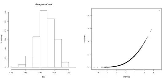
I made some simulations to illustrate. On the left, you see a histogram of the correlations for 1000 samples of 1000 pairs (X,Y) sampled such that the marginals are as above and they are comonotonic. What you see is that the sample correlation can be higher than $0.9031973$. But that is not unexpected. However the theoretical correlation is exactly $0.9031973$, as we computed above.

On the right, you see one sample of 1000 pairs (X,Y). You see that the dependence is indeed maximal. But precisely because it is not linear, the Pearson correlation is not well adapted to measure the degree of dependence.

Answer 2

I give you an illustration with the Gaussian copula, which I illustrated here as well.

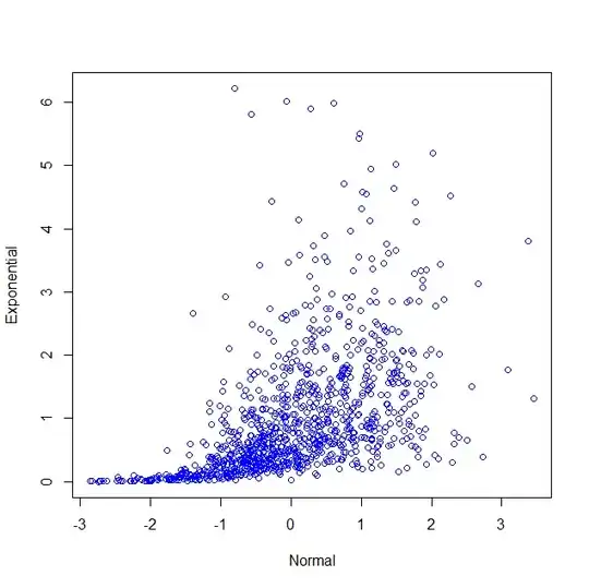
With the help of the package $\verb+copula+$ in R, I generate a bivariate distribution from a Gaussian copula with correlation parameter 0.54 and with marginals a standard normal and a standard exponential distribution ($\lambda=1$). My goal is correlation 0.5, but I take a slightly higher value to take into account the effect of my marginals.

library(copula)
joint.pdf <- mvdc(normalCopula(0.54), c("norm", "exp"),
          list(list(mean = 0, sd =1), list(rate = 1)))

par(mfrow=c(1,2))

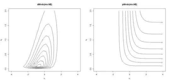
contour(joint.pdf, dMvdc, xlim = c(-4, 4), ylim=c(0, 2), main = "dMvdc(mv.NE)")
contour(joint.pdf, pMvdc, xlim = c(-4, 4), ylim=c(0, 2), main = "pMvdc(mv.NE)")

par(mfrow=c(1,2))

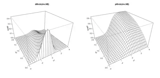
persp  (joint.pdf, dMvdc, xlim = c(-4, 4), ylim=c(0, 2), main = "dMvdc(mv.NE)")
persp  (joint.pdf, pMvdc, xlim = c(-4, 4), ylim=c(0, 2), main = "pMvdc(mv.NE)")

I plotted the contours of the density and cumulative distributions:

and made perspective plots as well:

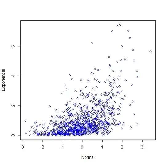
Finally, I generate a random sample of 1000 vectors and compute the sample Pearson correlation. I tried a few times to get the sample correlation close to 0.5. And I make a scatterplot.

data<-rMvdc(1000,joint.pdf);
cor(data);

par(mfrow=c(1,1))

plot(data,col='blue',xlab='Normal',ylab='Exponential')

The correlation I got is 0.5078836.

If you want to compute the theoretical Pearson correlation, you can use this formula in terms of the copula and the marginal distributions

$$\rho(X,Y)=\frac{1}{\sigma_X\sigma_Y}\int_0^1\int_0^1 (C(u,v)-uv)dF_X^{-1}(u)dF_Y^{-1}(v)$$

In our case, the marginals are of course those of the standard normal and the exponential, the $\sigma$'s are both 1 and the copula is

$$C(u,v)=\int_{-\infty}^{\phi^{-1}(u)}\int_{-\infty}^{\phi^{-1}(v)}\frac{1}{2\pi\sqrt{1-\rho^2}}\exp\left(-\frac{s_1^2-2\rho s_1s_2+s_2^2}{2(1-\rho^2)}\right)ds_1ds_2$$

Finally, I made one last scatterplot for which I selected a different copula, but kept the same marginals. I used a Clayton copula with parameter $\theta=1.8$.

$$C_{\theta}(u,v)=(u^{-\theta}+v^{-\theta}-1)^{-1/\theta}$$

It has the particularity that it has stronger dependence in the lower tail than in the higher tail of the distribution, which you can see clearly in the scatterplot, even though the sample correlation is only 0.5023782.