3

I have struggled with this a long time and haven't found an answer. I need to do a double lookup involving partially matching values. I need to return a certain value if my cell contains certain text.

For example, in the case shown below, I have a list of about 40,000 names in column A. In column D, I have a list of about 1,000 surnames. Each of the column A names contains one of these surnames. Column E contains a lookup value associated with each surname.

For each name in column A, I need to identify which column D surname it contains, and put that surname's associated value in column B.

For example, the name in A2 is A Smith. That contains Smith, which has an associated value of 3, so 3 would go in B2.

A3 also contains Smith, so B3 also gets the associated 3.

A4 contains White, which has an associated value of 4, so B4 gets 4.

A5 also contains White, so B5 also gets 4.

Ignore the coincidence of the column E values sometimes matching the column A row numbers. Also ignore the fact that capitalization in my example and explanation doesn't always match; in the actual data, all of the capitalization matches.

I tried to use =VLOOKUP(A2,"*"&B:C&"*",2,FALSE) but it did not work.

enter image description here

Addendum by fixer1234: As an abstract problem, this may still be confusing. Let me offer a common analogy.

Suppose in your community, every family has a different (i.e., unique) last name, and every member of a family shares the same last name. Each family lives together in the same house.

In column D, you have a list of the unique last names. In col E is the street address for the family with that last name. Columns D and E are a lookup table.

In column A is a list of everyone in the community. Each member of every family is in that list, but the names don't follow a standard format. Some are first name + last name, some are first initial + last name, some are last name + first name, etc. In column B, you want to put the street address for each person.

So the task is, for each column A name, find the last_name from column D that is contained in the column A name. From that last name, find the associated street address in column E, and return that to column B as the result. Since multiple members of each family are in the column A list, all of those family members will show the same resulting street address.

fixer1234
  • 27,486
  • Can you provide a little more detail? Roughly how many lookup values are there (like Smith and White)? What does the spreadsheet look like (add a screenshot)? What you want to do is a little bit the reverse of how VLOOKUP works, so the solution will be more complicated. There are a few ways to approach this and the number of lookup values would be a factor. Where does the result go (in a column next to each name, like 5 next to "A Smith", 4 next to "White B", etc.)? You show "white B" with a lowercase "w". Is that just a typo or do you need to match regardless of capitalization? – fixer1234 Apr 21 '19 at 22:55
  • Thank you for replying to me. I add a picture to my question hope it will make it more clear. The answers are needed in the next col. The "white" is just a typo. The number of lookups value is a lot, like 40000. The lookup array is about 1000. – Yujing Yang Apr 22 '19 at 05:36
  • @Scott, you're right, that's the same type of problem. Do you know if there are practical limits to the scale of an array (~1,000 virtual cells here)? – fixer1234 Apr 23 '19 at 16:29

1 Answers1

2

Your issue can be solved using Wildcard character:

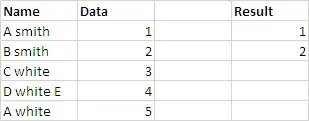
Example 1: When finding data of A smith:

enter image description here

Formula in Cell C2:

=IFERROR(VLOOKUP("A s*",A2:B6,2,FALSE),"")

Note, Excel considers Lookup value "A s*", A as first, SPACE second and s as third character, wrapped with Wildcard * which assumes more that one characters.

Example 2: When finding data of both A & B smith:

enter image description here

Formula in Cell D2:

=IFERROR(VLOOKUP("? s*",A55:B59,2,FALSE),"")

Note, Excel considers Lookup value "? s*", Wildcard ? for any one character, SPACE second and s as third character, wrapped with Wildcard * which assumes more that one characters.

Example 3: When finding data of C, D & A white.

enter image description here

An Array (CSE) Formula in Cell E2:

 {=IFERROR(INDEX($B$2:$B$6, SMALL(IF(ISNUMBER(SEARCH($F$1, $A$2:$A$6)), MATCH(ROW($A$2:$A$6), ROW($A$2:$A$6))), ROWS($A$1:A1))),"")}

N.B.

  • Finish this Formula with Ctrl+Shift+Enter and fill it down.
  • Cell F1 has match string.

Now let me explain how the Formula works:

SEARCH($F$1, $A$2:$A$6) becomes,

 SEARCH("white", {"A smith"; "B smith; C white"; "D white E"; "A white"})

ISNUMBER(SEARCH($F$1, $A$2:$A$6)) returns,

{FALSE; FALSE; TRUE; TRUE; TRUE}

Then combination of ISNUMBER, SEARCH and MATCH ROW becomes,

IF({FALSE; FALSE; TRUE; TRUE; TRUE}, {1; 2; 3; 4; 5})

and returns

{FALSE; FALSE; 3; 4; 5}

INDEX and SMALL sets Names and Filters nth smallest value, which finally finds Data 3,4 & 5 in adjacent cells of all whites.

Edited:

I've included this solution, responding addendum by @fixer1234 on OP, returns Common Numbers for each name match with Criteria.

Situation 1:

enter image description here


Situation 2:

enter image description here


Enter this Array (CSE) Formula in Cell B81, finish with Ctrl+Shift+Enter & fill it down.

{=IF($F$80="","",IF(ISNUMBER(SEARCH($F$80,A81:A$85)),INDEX($D$81:$E$82,SMALL(IF($D$81:$D$82=$F$80,ROW($D$81:$D$82)-80),1),2),""))}

N.B.

  • In this part ROW($D$81:$D$82)-80) -80 is editable, since the Formula is in Row 81, so you need to adjust it as your need.
  • Adjust cell references in the Formula as needed.
  • Cell F80 has Criteria which is case insensitive.
Rajesh Sinha
  • 9,218
  • 6
  • 17
  • 37
  • Nice tutorial material (+1) – Gary's Student Apr 22 '19 at 12:40
  • I agree, this is a great tutorial. But it doesn't actually solve what the OP wants to do. The requirement is the reverse. This solution starts with a single target name (White), finds all of the records in col A that contain it, and lists those record numbers for the target name. The OP wants to do it the other way around. There is a list of 1000 target names, each with an associated value. The OP wants to find, for each name in Col A, which of the 1000 target names is contained in the col A name, and put that target's associated value next to the col A name. – fixer1234 Apr 22 '19 at 20:28
  • @Gary'sStudent,, thanks for valuable observation ☺ – Rajesh Sinha Apr 23 '19 at 04:26
  • @fixer1234,, thanks for valuable observation,, the Screen Shot OP has attached are contradicting Source and Target data, in Col A name has two parts like A smith but in Col D OP expects Last name smith, since Col A has one more Smith,, so I think OP is little confused, therefore I've created sample data and suggested how to find single name and names in group also,, plz suggest how to make answer more effective. – Rajesh Sinha Apr 23 '19 at 04:37
  • You're right that the question was a bit confusing, and the OP didn't help by adding an example that didn't match the description. I did some edits in the question to clean it up and try to make it clearer. Read the edited question and see if it makes sense now. – fixer1234 Apr 23 '19 at 04:43
  • Cols D & E are a lookup table, not a result. The data is in col A, and the result goes in col B. The problem is a bit more complicated than it first appears. The name in col A must be found in col D, but it isn't a direct match. The match is the col D surname that is contained in the col A name. That's the twist that makes this one fun. – fixer1234 Apr 23 '19 at 04:49
  • @fixer1234, suppose Col D & E are lookup Table, then Source data in Col A is missing Number, in this case how both Name and Number can be used to match data in Col A !! – Rajesh Sinha Apr 23 '19 at 04:55
  • Right. The missing number is the problem the OP is trying to solve. The numbers are associated with the surnames in the lookup table (D&E). The task is to lookup the "full" name from col A against the surname list in col D to return the value from col E associated with the surname. The sticking point is that you can't do an exact match or even a typical partial match. The match is the col D name contained in the col A name. – fixer1234 Apr 23 '19 at 05:00