Generate rows based on columns

Question

I have a starting table like this:

And I need to generate a row for each of the letters in the third column. What I did so far is to extract that info into separate columns, like this:

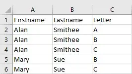
My goal is basically to get a table like this:

How can I achieve this? I thought about using a Pivot table, but I have no idea how and where to assign the different columns to in order to get what I need.

Note: I prefer not to use macros, as I have no experience using them, and I will have to do this kind of operation on a regular basis on different table structures, where the column "Letters" isn't as cut and dried as in my example (meaning I can't find out programmatically which row needs to be multiplied or not). I would have to rewrite the code constantly. I'd prefer if I could do it as a "regular" user.

I'm certain my method here https://superuser.com/questions/1185224/creating-multiple-rows-from-one-row-of-excel-data/1403367#1403367 can be adapted to this use case, but don't have time to write it out until tomorrow at the earliest. Give it a glance, and/or I'll try to remember to come back — Alex M, Feb 20 '19 at 01:47

score 0 · Answer 1 · answered Feb 19 '19 at 15:30

If you start with this on Sheet1:

and run this macro:

Sub MakeReport()
    Dim k As Long, i As Long, N As Long, s1 As Worksheet, s2 As Worksheet
    Dim v1 As String, v2 As String, lt As String, L As Long, ll As Long

    Set s1 = Sheets("Sheet1")
    Set s2 = Sheets("Sheet2")
    N = s1.Cells(Rows.Count, "A").End(xlUp).Row
    k = 1
    For i = 2 To N
        v1 = s1.Cells(i, 1).Value
        v2 = s1.Cells(i, 2).Value
        lt = s1.Cells(i, 3).Value
        L = Len(lt)
        For ll = 1 To L
            s2.Cells(k, 1) = v1
            s2.Cells(k, 2).Value = v2
            s2.Cells(k, 3) = Mid(lt, ll, 1)
            k = k + 1
        Next ll
    Next i
End Sub

You will get this on Sheet2:

Thanks for the answer, but I prefer if I didn't have to use macros (see edit). — , Feb 19 '19 at 15:39

Ron Rosenfeld · Accepted Answer · 2019-02-20T12:13:07.010

Edit: Screenshots added to assist in finding option locations

Use Get&Transform from the Data tab. Select From Table/Range

The Power Query user interface will open
Select the Letters Column and the option to Split Column by number of Characters (where the number of characters is one (1)).

Select the Firstname and Lastname columns
Select to UNpivot other columns.

Delete the Attribute column created after the Unpivot.

Close and Load

After you've done this once, you can add data to the table and re-run the query, if necessary.

Generate rows based on columns

2 Answers2