The conic curves you consider undergo four constraints : all of them pass through the 2 points $(0,-1)$ and $(0,1)$ and are tangents in those points to the 2 lines with resp. equations $y=-1$ and $y=1$.
This kind of family of conics is called a bitangent linear pencil. The curves belonging to this pencil can be given the general equation :
$$ax^2+y^2-1=0 \ \ \ \begin{cases}a>0& \ \text{ for ellipses}\\a<0& \ \text{ for hyperbolas}\\a=0& \ \ \text{for the pair of lines}\end{cases} \tag{1}$$
Remark : Equation (1) relies on a single parameter $a$, a "degree of freedom". How could it be foreseeable ? Very simply : a conic curve is determined by $5$ conditions (passing through $5$ points, or being tangent to $5$ lines or any "mixture" between those conditions), it remains $5-2-2=1$ degree of freedom.
I am going to give two methods, the second one (have a look at the second figure) providing a definitive answer. The first one is a numerical method (almost always possible for obtaining orthogonal curves) giving a satisfying graphical answer but no more.
First method (numerical solution) :
First of all, we re-write (1) under the form :
$$\frac{1-y^2}{x^2}=a\tag{2}$$
In order that, when (2) is differentiated this with respect to $x$, parameter $a$ disappears :
$$\frac{-2yy'x^2-(1-y^2)2x}{x^4}=0\tag{3}$$
(3) can be considered as equivalent to :
$$y'=\frac{y^2-1}{xy}\tag{4}$$
which is the ordinary differential equation (ODE) common to all curves of the pencil of conics.
The ODE common to all orthogonal curves is obtained by replacing $y'$ in the expression above by $-\frac{1}{y'}$ (the product of slopes in any point $(x,y)$ must be $-1$) giving :
$$y'=\frac{xy}{1-y^2}\tag{5}$$
Numerical solutions of (5) can be obtained (see blue curves below) with a code in any scientific programming language having an ODE solver. I have done it with Matlab.
Some numerical inaccuracies occur around line $y=1$ ; they are due to the $1-y^2$ denominator in (5).
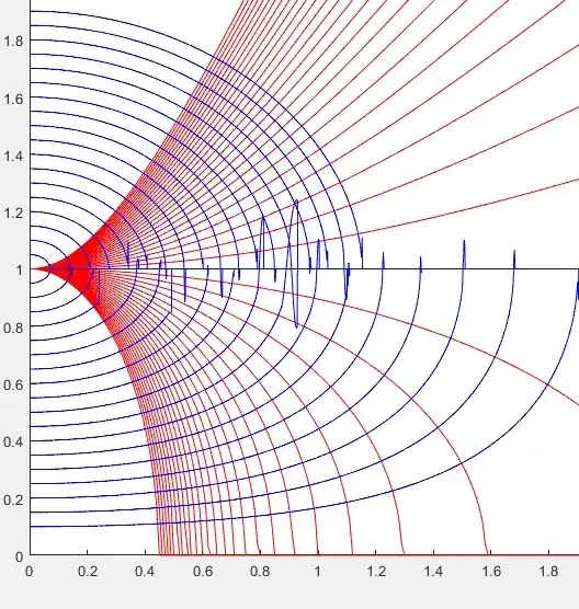
Fig. 1 : Representation of the solutions in the first quadrant, WLOG because the issue is symmetrical with respect to the $x$ and $y$ axes.
Second method : (rigorous approach ; see Fig. 2).
The set of orthogonal functions is given by equations
$$y=\sqrt{-W(n,-ke^{x^2})} \tag{6}$$
where $W$ is the Lambert function (with $n=0$ or $n=-1$), depending on the arbitrary positive constant $k$.
Proof of (6) in the case of the principal branch ($n=0$) :
We will abbreviate (it is classical) $W(0,x)$ into $W(x)$.
Function $W$ is known to verify the following differential equation :
$$\frac{W'(u)}{W(u)}=\frac{1}{u(1+W(u))}\tag{7}$$
Besides, as (6) can be written under the form :
$$\ln y = \frac12 \ln(-W(-ke^{x^2}))$$
Its differentiation gives :
$$\frac{y'}{y}=\frac12 \frac{-W'(-ke^{x^2})(-2kxe^{x^2})}{W(-k e^{x^2})}$$
Now use relationship (7) with $u=-k e^{x^2}$ in order to show that (5) is verified.

Fig. 2. Ellipses, Hyperbolas, and the two families of orthogonal curves with resp. colors red, magenta, green and blue.
Fig. 2 has been obtained with the following SAGE program implementing the $W$ function :
 var('x y')
 g=line([[0,-2.5],[0,2.5]],color='black',aspect_ratio=1,); # axes etc.
 g+=line([[-2,0],[2,0]],color='black')
 g+=plot(1,(x,-2,2),color='red')
 g+=plot(-1,(x,-2,2),color='red')
 for k in range(5):
    a=(k+1)/2;
    g+=implicit_plot(a*x^2+y^2-1,(x,-2,2),(y,-1,1),color='red'); # ellipses
    g+=implicit_plot(-a*x^2+y^2-1,(x,-2,2),(y,-2.5,2.5),color='magenta'); # hyperbolas
 v(x,p,b)=sqrt(-lambert_w(p,-b*exp(x^2)))
 r=1.8;
 for k in range(6):
    b=(k+1)/40
    g+=plot(v(x,0,b),(x,-r,r),color='green',plot_points=3000)
    g+=plot(v(x,-1,b),(x,-r,r),color='blue',plot_points=3000)
 g


