Alright, sorry for the delayed response. My comments on AIC and BIC, while if applied correctly will work, were not helpful to reaching a conclusive answer, which I try to give when I comment or answer. I'm not an expert on information criteria like those, but I know they are used somewhat often which is why I suggested them. Hopefully the following discussion will be more practical, as it is specifically geared towards AR models.
AR models are all-pole white noise generative models, which means that the current value in the time series can be predicted as a linear combination of its previous $p$ values plus a stochastic input term. This is mathematically described as
\begin{equation} x_{n} = a_{1}x_{n-1} + a_{2}x_{n-2} + \dots + a_{p}x_{n-p} + w_{n} \end{equation}
In order to delve into the basics of model order selection, we need to understand the autocorrelation function (ACF) and partial autocorrelation function (PACF), specifically of AR models. The autocorrelation function is pretty well known, and practically is found by a time-averaged estimate of
\begin{equation}E[x(n)x^{*}(n-m)]\end{equation}
The autocorrelation function of an AR process typically exhibits erratic behavior that slowly tapers towards zero as you move away from the central point. Conceptually this makes sense. The current value in an AR series is dependent on the previous $p$ values, but each of those previous values are dependent on their own respective sets of previous $p$ values! So, the autocorrelation function will have somewhat erratic behavior that doesn't settle quickly.
On the other hand, the PACF measures the correlation between the current value $n$ and the lagged value $n-k$ while removing the effects of the intervening lags. That is to say, it measures the direct effect of each lagged value on the current value. This is important because the AR model assumes that there are only $p$ previous values, so the PACF should theoretically be zero for all values greater than $p$.
What this means is that we should expect the PACF to be zero after a certain number of values (to within a confidence interval), and the number of values whose magnitude is greater than this confidence interval should be the model order. I believe most, if not all, of Matlab's AR parameter estimation functions have the ability to return reflection coefficients, of which the PACF is the negation of. You can use this link to see how to perform this in Matlab.
Now, for this specific case, ie multiple sinusoids (potentially in noise) that form a line spectrum, you will likely see that both the ACF and PACF have decaying oscillatory behavior. This is because this signal model exhibits strong periodicity (I believe this is referred to as seasonality by time series people). This means that, in order to get really accurate extrapolation, you will likely need an ARMA model of some sort. But, Burg's should at least give you a reasonable estimate. You'll want to take the first value that dips below the confidence interval as "optimal", which I found to give roughly an order of $p=23$ with my testing.
Hopefully this helps!
**EDIT #1: **
Per request in the comments, here is how I came to the conclusion of what model order to use.

As can be seen in the picture, the PACF dips below the confidence interval at the value highlighted in red. This is the 24th value in the sequence, so we use 23 as our model order. The code I used is shown below.
N = 150;    % Order of LPC auto-regressive model
P = 500;    % Number of samples in the extrapolated time series
M = 200;    % Point at which to start predicting
t = 1:P;
x1 = 5sin(t/3.7+.3)+3sin(t/1.3+.1)+2*sin(t/34.7+.7); % This is the measured signal
x0 = x1;
x1(M+1:end) = 0;
[~,~,k] = arburg(x0(1:M),M-1);
pacf = -k;
figure;
stem(pacf,'filled');
xlim([1 50]);
conf = sqrt(2)erfinv(0.95)/sqrt(M);
hold on;
plot(xlim,[1 1]'[-conf conf],'r');
hold off;
p = input("Enter the first x-axis value where the PACF magnitude drops to within the confidence interval: ");
a = arburg(x0(1:M),p-1);
y1 = zeros(1, P);
% fill in the known part of the time series
y1(1:M) = x1(1:M);
% in reality, you would use filter instead of the for-loop
for ii=(length(a)):P

    y1(ii) = -sum(a(2:end) .* y1(ii-1:-1:ii-length(a)+1));
end
figure;
plot(t, x0,'b', t, x1,'or', t, y1,':xk','LineWidth',1);
l = line(M*[1 1], get(gca, 'ylim'));
set(l, 'color', [0,0,0]);
legend('expected signal prediction', 'actual signal', 'extrapolated signal', 'start of extrapolation');
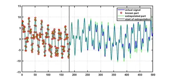
This using a value of $p=24$ produces the following output


xthat has only N elements ? do I keep the point where to start predicting the same ? – bla Mar 08 '24 at 20:24