How to improve my FFT output?

Question

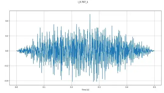
I am to reproduce the figure below but with a different blue line (source), which shows the ideal normalized frequency spectrum (grey) of a spectral ripple with 0.7 ripple-per-octave and an electric spectrum of a speech coding strategy. Below you can find the time signal of the spectral ripple sound. Unfortunately, the sound is only half a second so I understand the frequency resolution I can achieve with a sampling frequency of 44100 Hz is 2 Hz (Fs/num_samples = 44100/22050)

I have several questions on how to achieve this (in python):

1. Why does my frequency spectrum show such "spiky" behaviour instead of a sinusoid as the first figure?

import numpy as np
from scipy.io import wavfile
import matplotlib.pyplot as plt
Fs, audio_signal_single = wavfile.read(sound_name) # Fs = 44100
FFT = np.fft.rfft(audio_signal)
abs_fourier_transform = np.abs(FFT)
power_spectrum = np.square(abs_fourier_transform)
frequency = np.linspace(0, Fs/2, len(abs_fourier_transform))
max_power = power_spectrum.max()
normalized_power = power_spectrum/max_power
plt.plot(frequency, np.squeeze(normalized_power), color='grey')

2. I thought about zero padding, but I read this does not improve the frequency resolution ["zero padding can lead to an interpolated FFT result, which can produce a higher display resolution."] 5 But I'm not really sure what this entails, but with 22050 samples and zero padding up to 2^15 I think this would give an (interpolated) resolution of 0.67 Hz. Why does it seem that the spectrum is shifted to the left? Am I right to skip zero padding to improve my figure? Similarly, I tried repeating the signal, but this also seemed to distort the spectrum and I read here that this also does not help.

FFT = np.fft.fft(audio_signal, 2**15)

3. I have applied a blackman-hanning window prior to performing the FFT, but I noticed this only affects this spiking in the lower frequencies. Why is this? How can I extend this effect to higher frequencies?

window = 0.5 * (np.blackman(len(audio_signal)) + np.hanning(len(audio_signal))) 
audio_signal *= window

4. I don't recall FFT having an effect on the power in higher frequencies, why does the power decrease with higher frequency in my image? How can I counter this? I have applied a pre-emphasis filter which slightly helps, but is there a better solution? Why is the spectrum suddenly cut-off? This could have been present before, but the power was too small to notice.

audio_signal = scipy.signal.lfilter(coeff_numerator, coeff_denominator, audio_signal)

In short, is there a way I can improve my spectral output to make it more similar to the image I am trying to replicate?