Determining Frequency and Period of a wave

Question

I'm gathering temperature data from a refrigerator. The data looks like a wave. I would like to determine the period and frequency of the wave (so that I can measure if modifications to the refrigerator have any effect).

I'm using R, and I think I need to use an FFT on the data, but I'm not sure where to go from there. I'm very new to R and signal analysis, so any help would be greatly appreciated!

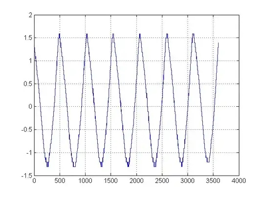
Here is the wave I'm producing:

Here is my R code so far:

require(graphics)
library(DBI)
library(RSQLite)

drv <- dbDriver("SQLite")
conn <- dbConnect(drv, dbname = "s.sqlite3")

query <- function(con, query) {
  rs <- dbSendQuery(con, query)
  data <- fetch(rs, n = -1)
  dbClearResult(rs)
  data
}

box <- query(conn, "
SELECT id,
       humidity / 10.0 as humidity,
       temp / 10.0 as temp,
       ambient_temp / 10.0 as ambient_temp,
       ambient_humidity / 10.0 as ambient_humidity,
       created_at
FROM measurements ORDER BY id DESC LIMIT 3600
")

box$x <- as.POSIXct(box$created_at, tz = "UTC")

box$x_n <- box$temp - mean(box$temp)
png(filename = "normalized.png", height = 750, width = 1000, bg = "white")
plot(box$x, box$x_n, type="l")

# Pad the de-meaned signal so the length is 10 * 3600
N_fft  <- 3600 * 10
padded <- c(box$x_n, seq(0, 0, length= (N_fft - length(box$x_n))))
X_f    <- fft(padded)
PSD    <- 10 * log10(abs(X_f) ** 2)

png(filename = "PSD.png", height = 750, width = 1000, bg = "white")
plot(PSD, type="line")

zoom <- PSD[1:300]

png(filename = "zoom.png", height = 750, width = 1000, bg = "white")
plot(zoom, type="l")

# Find the index with the highest point on the left half
index <- which(PSD == max(PSD[1:length(PSD) / 2]))

# Mark it in green on the zoomed in graph
abline(v = index, col="green")

f_s     <- 0.5 # sample rate in Hz
wave_hz <- index * (f_s / N_fft)
print(1 / (wave_hz * 60))

I've posted the R code along with the SQLite database here.

Here is a plot of the normalized graph (with the mean removed):

So far, so good. Here is the spectral density plot:

Then we zoom in on the left side of the plot and mark the highest index (which is 70) with a green line:

Finally we calculate the frequency of the wave. This wave is very slow, so we convert it to minutes per cycle, and print out that value which is 17.14286.

Here is my data in tab delimited format if anyone else wants to try.

Thanks for the help! This problem was hard (for me) but I had a great time!

Answer 1

Interesting project you have going on there! :-)

From a signal analysis POV, this is actually a simple question - and yes, you are right that you would utilize the FFT for this frequency estimation problem.

I am not familiar with R, but what you essentially want to do is take the FFT of your temperature signal. Since your signal is real, you will get a complex result as the output of your FFT. You can now take the absolute magnitude squared of your complex FFT result, (since we dont care about phase). That is, $real^2 + imag^2$. This is your power spectral density.

Then, very simply, find the max of where your PSD sits. The abscissa of that max will correspond to your frequency.

Caveat Emptor, I am giving you a general outlook, and I suspect the result of the FFT in R will be normalized frequency, in which case you would have to know your sample rate, (which you do), in order to convert it back into Hz. There are many other important details that I am leaving out, such as your frequency resolution, FFT size, and the fact that you probably want to de-mean your signal first, but it will be good to see a plot first.

EDIT:

Let us take your signal into account. After I de-mean it, it looks like this:

You want to de-mean because the DC bias is a frequency of 0 Hz technically, and you do not want it to drown out other frequencies of interest. Let us call this de-meaned signal $x[n]$.

Now, when you take the FFT, you must take heed of some details. I use an FFT length of 10 times the length of the signal, so we can say that $N_{fft} = 10 * 3600 = 36000.$ Any FFT size set greater than the size of the original signal has the effect of interpolating your FFT result in the frequency domain. While this doesnt add any information for you from an information theory POV, it does help you better discern where exactly your true peak lies, especially in cases where it lies between two frequency bins. To get true better frequency resolution, you want to get more data. (i.e, let the sensor run for a longer period of time).

Moving along, from the text file, I see that your sensor is taking temperature readings every 2 seconds. This means that your sampling rate, or $f_s = 0.5 Hz$

Thus, let us take an FFT of $x[n]$, and call that result $X(f)$. This result will be complex, and in fact, it is conjugate symmetric, but thats not important here. (It just means for your purposes, half of it is redundant). Now if we take $10log_{10}(|X(f)|^{2})$, this is the power spectral density (in log scale). The result looks like so:

You can see how it is symmetric. If you ignore the last half, and just look at the first half and zoom in you, can see this:

So you have a peak at index 70! But what is index 70 in real frequency terms? Here is where you want your frequency resolution. To compute that, we simply take $\frac{F_s}{N_{fft}} = 1.3889e-005 Hz$. This simply means that every index represents a frequency that is a multiple of this number. Index 0 is $0 * 1.3889e-005 = 0 Hz$. Index 1 is $1 * 1.3889e-005 = 1.3889e-005 Hz$. Index 70 is $70 * 1.3889e-005 = 9.7222e-004 Hz$.

We are almost done. Now that you have this figure, we can convert it to something more palatable. This figure is just saying that your signal completes 9.7222e-004 cycles every second. So we can ask, how many minutes does it take to compute one cycle? Thus, $\frac{1}{(9.7222e-004)*60} = 17.14$ minutes per cycle.

Answer 2

There is no need to do anything complicated: just measure the duration between peaks of the waveform. This is the period. The frequency is just 1 divided by the period.

With about 8 cycles over 2 hours, the frequency is 4 cycles per hour, or about 1 mHz.

Answer 3

For a waveform this smooth and stationary, counting sample points between positive going crossings of some average threshold value will give you a period estimate. Look at several threshold crossing periods to get a more average estimate or detect any trend.